前言
Cartopy 是为了向 Python 添加地图制图功能而开发的扩展库。该项目致力于以 matplotlib 包为基础,用简单直观的方式操作各类地理要素的成图。Cartopy 官网的画廊页面已经提供了很多绘图的例子,它们和官方文档一起,是学习该工具的主要材料。
绘制 IGS 站点分布图
本图使用的 IGS 核心站与 MGEX 项目站点,及其坐标均来自 IGS 网站。我已经将其整理成为 igs-core 和 mgex 两个 CSV 文件,你可以直接下载。
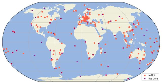
IGS 核心站与 MGEX 站点分布图
import numpy as np
import matplotlib.pyplot as plt
import cartopy.crs as ccrs
import cartopy.feature as cfeature

# Load the coordinate of IGS Core & MGEX sites, The CSV files are
# exported from: http://www.igs.org/network
igs_core = np.recfromcsv('igs-core.csv', names=True, encoding='utf-8')
mgex = np.recfromcsv('mgex.csv', names=True, encoding='utf-8')

fig = plt.figure(figsize=[9, 6])
# Set projection
ax = plt.axes(projection=ccrs.Robinson())
# Add ocean and land
ax.add_feature(cfeature.LAND)
ax.add_feature(cfeature.OCEAN)
# Add MGEX & IGS core sites
ax.plot(mgex['longitude'], mgex['latitude'], 'o', color='tomato',
        label='MGEX', transform=ccrs.Geodetic())
ax.plot(igs_core['longitude'], igs_core['latitude'], '*', color='darkmagenta',
        label='IGS Core', transform=ccrs.Geodetic())
# Plot gridlines
ax.gridlines(linestyle='--')
# Set figure extent
ax.set_global()
# Set legend location
plt.legend(loc='lower right')
# Show figure
plt.show()
PS:如有需要Python学习资料的小伙伴可以加下方的群去找免费管理员领取

可以免费领取源码、项目实战视频、PDF文件等
绘制 GNSS 控制网
这里使用的 IGS 站点坐标数据同样来自 IGS 网站。我已将其整理成一个 CSV 格式的文件:euro-igs,你可以直接下载使用。这里使用 matplotlib.tri 中的 Triangulation 来根据输入的点位坐标来创建 Delaunay 三角网,然后使用 plt.triplot() 方法绘制。
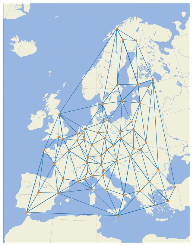
GNSS 控制网
import numpy as np
import matplotlib.pyplot as plt
import matplotlib.tri as tri
import cartopy.crs as ccrs
import cartopy.feature as cfeature

# Load coordinate of the IGS sites in Europe, this CSV file is
# exported from: http://www.igs.org/network
igs_sites = np.recfromcsv('euro-igs.csv', names=True, encoding='utf-8')
# Generate Delaunay triangles
triangles = tri.Triangulation(igs_sites['longitude'], igs_sites['latitude'])

fig = plt.figure(figsize=[6, 8])
# Set projection
ax = plt.axes(projection=ccrs.LambertConformal(central_latitude=90,
                                               central_longitude=10))
# Add ocean, land, rivers and lakes
ax.add_feature(cfeature.OCEAN.with_scale('50m'))
ax.add_feature(cfeature.LAND.with_scale('50m'))
ax.add_feature(cfeature.RIVERS.with_scale('50m'))
ax.add_feature(cfeature.LAKES.with_scale('50m'))
# Plot triangles
plt.triplot(triangles, transform=ccrs.Geodetic(), marker='o', linestyle='-')
# Plot gridlines
ax.gridlines(linestyle='--')
# Set figure extent
ax.set_extent([-10, 30, 30, 73])
# Show figure
plt.show()
绘制板块分布图
板块构造理论将地球的岩石圈分为十数个大小不等的板块。本图使用的 Nuvel 板块边界数据来自 EarthByte 网站,我已经将其整理为一个压缩文件,你可以直接下载使用。
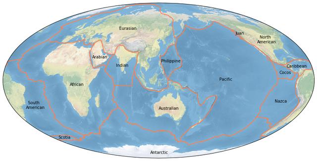
Nuvel 板块分布图
import numpy as np
import matplotlib.pyplot as plt
import cartopy.crs as ccrs

# The plate boundary files
files = ['African.txt', 'Antarctic.txt', 'Arabian.txt', 'Australian.txt',
         'Caribbean.txt', 'Cocos.txt', 'Eurasian.txt', 'Indian.txt', 'Juan.txt',
         'Nazca.txt', 'North_Am.txt', 'Pacific.txt', 'Philippine.txt',
         'Scotia.txt', 'South_Am.txt']
# Read boundaries into numpy
borders = []
for f in files:
    border = np.genfromtxt(f, names=['lon', 'lat'], dtype=float, comments=':')
    borders.append(border)
# Plate names
plates = ['African', 'Antarctic', 'Arabian', 'Australian', 'Caribbean', 'Cocos',
          'Eurasian', 'Indian', 'Juan', 'Nazca', '  North\nAmerican', 'Pacific',
          'Philippine', 'Scotia', '  South\nAmerican']
# Central point for every plate, just for text positioning
central = [(17, -5), (90, -80), (40, 21), (120, -28), (270, 12), (260, 6),
           (60, 50), (70, 13), (230, 45), (260, -21), (250, 36), (190, 0),
           (123, 17), (304, -59), (315, -27)]

# Start plot
fig = plt.figure(figsize=(12, 7))
ax = plt.axes(projection=ccrs.Mollweide(central_longitude=120))
# Plot a image as background
ax.stock_img()
# Plot boundaries
for plate, center, border in zip(plates, central, borders):
    ax.plot(border['lon'], border['lat'], color='coral',
            transform=ccrs.Geodetic())
    ax.text(center[0], center[1], plate, transform=ccrs.Geodetic())

plt.show()
本文的文字及图片来源于网络,仅供学习、交流使用,不具有任何商业用途,版权归原作者所有,如有问题请及时联系我们以作处理。
以下文章来源于EasyShu ,作者姜英明